The 15.6x Memory Hack: How to Run Knowledge Distillation on a Single GPU

A 20-billion-parameter distillation that needed four GPU nodes now runs on one. Step time dropped from 57 seconds to 12.2 seconds. Peak memory fell from roughly 250 gigabytes to 128 gigabytes on a single H200. Not a new model. Not a new chip. A new way to handle the teacher's output during distillation. Here is how it works and why it changes what your team can afford to compress.

The Memory Wall: Why Distillation Breaks at Scale

Distillation requires both teacher and student models in memory simultaneously, plus a full vocabulary-by-sequence probability distribution. At 32,000 tokens, the dense KL loss in a controlled microbenchmark peaks at 85.2 GiB. The fused chunked version peaks at 5.45 GiB. That is a 15.6x reduction at the kernel level, and the dense loss fails outright beyond 64,000 tokens. In the real world, distilling GPT-OSS-20B at 32K context, the dense loss spikes to roughly 250 GB, which exceeds a single H200's 141 GB capacity. The fused chunked loss peaks at about 128 GB, which fits.

Here is why it explodes. Standard distillation computes the teacher's full probability distribution across the entire vocabulary for every token in the sequence. Vocabulary size times sequence length times float precision equals a matrix nobody can hold. At 32K tokens with a vocabulary of 131,072 entries, that tensor alone is the memory killer. Teams that want to distill a frontier model into a deployable size need multi-node GPU clusters just for the distillation run, before they even start training the student. That cost has been the gating factor.

The Offline Caching Trick: Why the Teacher Never Sits in Memory

The first fix is simple in concept and brutal in impact. Cache the teacher's top-K logits once, offline. The teacher model is never loaded alongside the student during training. The only thing in memory is the pre-computed logits for the relevant tokens.

Here is how it works. Run the teacher once over the entire dataset. For every token position, store only the 100 largest logits and their probabilities. During student training, load those cached values instead of running the teacher forward pass. The Multiverse Computing team showed this matches online distillation at near-identical training loss while cutting peak memory and raising throughput by about 40 percent on a single H200.

Implementation for Top-K Logits Caching

import torch
from transformers import AutoModelForCausalLM, AutoTokenizer
from datasets import load_dataset
import safetensors.torch as st

def cache_teacher_logits(model_id, dataset_name, k=100, output_path="teacher_topk.safetensors"):
    # Load teacher in FP16 to save VRAM during the offline pass
    model = AutoModelForCausalLM.from_pretrained(model_id, torch_dtype=torch.float16, device_map="cuda")
    tokenizer = AutoTokenizer.from_pretrained(model_id)
    dataset = load_dataset(dataset_name, split="train")
    
    cache = {}
    for i, example in enumerate(dataset):
        inputs = tokenizer(example["text"], return_tensors="pt").to("cuda")
        with torch.no_grad():
            logits = model(**inputs).logits # Shape: [seq_len, vocab_size]
            # Extract the top K values and their corresponding indices
            vals, idxs = torch.topk(logits, k=k, dim=-1)
            
            # Store as tensors for each token in the sequence
            for j in range(logits.shape[0]):
                cache[f"token_{i}_{j}"] = {
                    "values": vals[j].cpu(), 
                    "indices": idxs[j].cpu()
                }
    
    st.save_file(cache, output_path)

Why top-100 is sufficient: the vast majority of the probability mass concentrates in the top logits. The long tail contributes negligibly to the KL divergence signal. The retained mass may be strictly below one because of truncation, but the formulation accounts for the partial mass exactly. Removing the teacher from the training loop eliminates the largest single memory consumer in the distillation pipeline.

The Fused Chunked KL Loss: Killing the Vocabulary Matrix

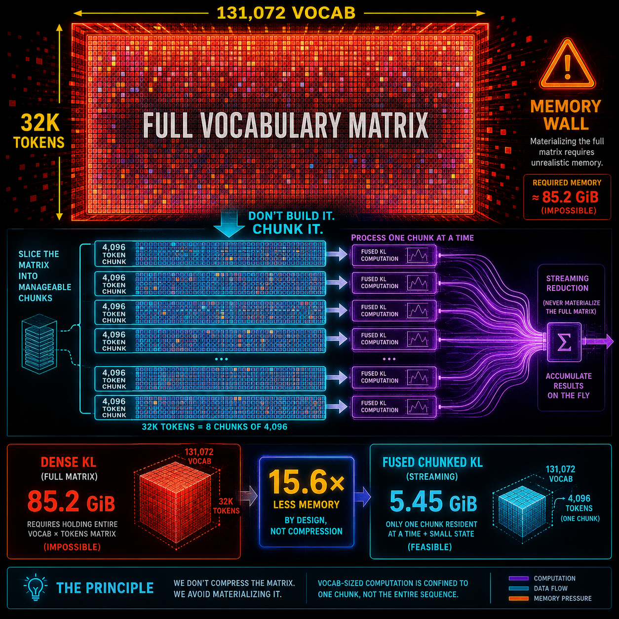
The second fix attacks the vocabulary-sized tensor itself. A fused chunked KL loss processes the vocabulary dimension in chunks, never materializing the full vocabulary-by-sequence matrix in memory at once.

The standard approach requires computing the full probability distribution across the entire vocabulary for every token. That matrix is the memory killer. The chunked approach processes the sequence in segments of 4,096 tokens. Each chunk computes its own normaliser, accumulates the sparse teacher terms, and immediately discards the logits. In the backward pass, the logits are recomputed chunk by chunk, the softmax is rebuilt from the saved normaliser, and the gradient is formed in closed form. The vocabulary-sized cost is confined to a single chunk and is independent of sequence length. The only quantity that grows with longer sequences is the hidden-state activation, which is tiny by comparison.

Implementation for Fused Chunked KL Loss

import torch

def chunked_kl_loss(teacher_logits, student_logits, chunk_size=4096):
    vocab_size = teacher_logits.shape[-1]
    total_kl = 0.0
    
    # Process the vocabulary dimension in manageable chunks
    for start in range(0, vocab_size, chunk_size):
        end = min(start + chunk_size, vocab_size)
        
        # Slice the vocabulary dimension
        t_chunk = teacher_logits[:, start:end]
        s_chunk = student_logits[:, start:end]
        
        # Compute the KL divergence for the current chunk
        # Log-softmax is computed on the slice and normalizer is handled via fused kernel
        chunk_loss = torch.nn.functional.kl_div(
            torch.log_softmax(s_chunk, dim=-1),
            torch.softmax(t_chunk, dim=-1),
            reduction="sum"
        )
        total_kl += chunk_loss
        
    return total_kl / teacher_logits.shape[0]

The fused aspect means the output projection and the loss computation happen in a single kernel pass, avoiding intermediate storage. The result: at 32K tokens in the isolated benchmark, peak memory drops from 85.2 GiB to 5.45 GiB. At 64K tokens, where the dense loss runs out of memory, the chunked version still runs. At 256K tokens, the fully chunked loss holds at 11.6 GiB while the forward-chunked variant (which still keeps full logits in memory) hits 134.2 GiB.

The Real-World Result: Four Nodes to One, 57 Seconds to 12.2

In the GPT-OSS-20B distillation at 32K context on eight H200 GPUs, the memory freed by the fused chunked loss let the setup drop from four nodes to a single node. Step time fell from 57.0 to 12.23 seconds. Throughput per GPU rose from 74.2 to 345.7 TFLOP per second. The total compute cost of a distillation run drops by roughly 18x. That is not optimization. That is a category change.

The resulting compact student, derived from Llama 3.1 8B Instruct, retains most of the teacher's accuracy at less than half the parameter count. On BoolQ and HellaSwag, the gap is about one to two points. On MMLU, it is about nine points. On WinoGrande and GSM8K, the gap widens to about eleven and twelve points respectively. Instruction following and factual recall transfer well. Complex reasoning and edge-case mathematics degrade more noticeably. The trade-off is real, and it is specific to the task.

If you were priced out of distillation because you needed a multi-node cluster, the barrier just moved. One node. One GPU in many configurations. That changes who can afford to run this pipeline.

Why This Matters Now: The Frontier Model Size Problem

Kimi K3 is a 2.8-trillion-parameter open-weight model. At FP16 precision, it needs roughly 5.6 terabytes of VRAM just to load the weights, excluding KV cache. At FP8, it still needs about 2.8 TB. You cannot deploy that on standard infrastructure. You must distill it into something smaller.

Frontier models are growing faster than deployment infrastructure can absorb. Distillation is the bridge between frontier capability and deployable reality. The constraint was never whether you can train a small model. It was whether you can afford the distillation run. This technique moves that constraint.

Intelligence per dollar is the metric that decides which stacks survive. This technique directly improves that ratio by an order of magnitude. That is not a marginal improvement. That is a structural shift in who can build competitive models.

What to Do Today

If you are distilling a model, implement offline top-K logits caching before your next run. The teacher model should never be in memory during student training. If you are evaluating distillation frameworks, ask whether they support chunked KL loss. If they materialize the full vocabulary matrix, they will fail at long context lengths. If you are planning a model compression pipeline, the old assumption was that distillation needs a cluster. The new assumption is that distillation needs a node. Recalculate your budget. If you are building on a frontier model you cannot deploy at full size, this technique makes distillation practical enough to be your deployment strategy, not a research project.

The Uncomfortable Question

If a 3.2 billion parameter student can retain most of an 8 billion parameter teacher's accuracy at less than half the parameters, and the distillation run costs 18x less than it did last month, what is your excuse for still calling the cloud API? The barrier to owning your model has never been lower. The barrier to justifying the cloud bill has never been higher.