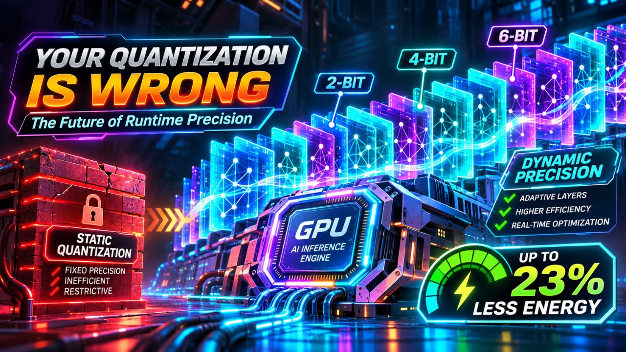
You picked a quantization level once, at deploy time, and it has been wrong for most of your layers ever since. A paper posted to arXiv on November 6 puts a number on that habit. The same accelerator design, running precision as a runtime decision instead of a build-time constant, cuts energy by up to 23 percent and latency by up to 2.3 times at identical accuracy.
The paper is AutoEMatic, from Akshat Ramachandran and six co-authors across Georgia Tech and NVIDIA, and the numbers are not subtle. Up to 21.7 percent accuracy improvement over NVFP4 across reasoning and agentic benchmarks, group-scaled FP6 accuracy on most of those benchmarks at 4.9 bits per weight (an effective average across selectively refined subgroups) against 4.5 for NVFP4, and 90 to 98 percent of NVFP4 decode throughput on GB300 GPUs. That is not a trade, it is a refund.
One caveat belongs on the first screen, before the numbers do the selling. The energy and latency figures come from a simulated accelerator with an AutoFP-native datapath, measured against the same design limited to an NVFP4 datapath at matched accuracy, so they are a hardware-class argument, not a number you collect by upgrading vLLM tomorrow. And we already covered why your decode phase is memory bound in "Your Decode Phase Is Memory-Bound. Speculative Decoding Is the Fix." This is the next domino. If bandwidth is the constraint, precision decides how much of it you waste.
THE STATIC QUANTIZATION TRAP
Every post-training quantization pipeline you have built follows the same shape. Train the model, run a calibration pass, choose a format, pin it, ship it. The paper's own baselines calibrate on 256 samples from WikiText-2 and then hold that assignment for the life of the deployment.
That is a fixed policy applied to a moving target. Precision demand changes with the prompt, between prefill and decode, and from one step to the next. The paper's motivating measurement shows the precision distribution shifting across early, middle and late stages of a single request. A layer that is easy at step 5 can be the sensitive one at step 50.
The economics run in one direction. A static assignment over-provisions precision where it is not needed and under-provisions it where it is, and both halves cost you. The over-provisioned half is energy and latency you burn on work that never needed the bits. The under-provisioned half shows up as accuracy you never see, because you measured it once and called the number final.
A model doing routine extraction does not need what a hard reasoning pass needs. Set the number once and you pay peak cost for floor-level workloads all day.
This is not the compress-then-heal story from "Your 4-Bit Model Just Beat Its Full-Precision Original. The Compress-Then-Heal Pipeline Is Broken." That piece was about repairing damage after quantization. This one is about never committing to one precision that long.
THE PRECISION CONTROL LOOP
Here is the framework worth naming and reusing: the Precision Control Loop. It is a control loop, not a compression setting. Compression is a decision about a file. Control is a decision about a running system, on a schedule, from measurements.
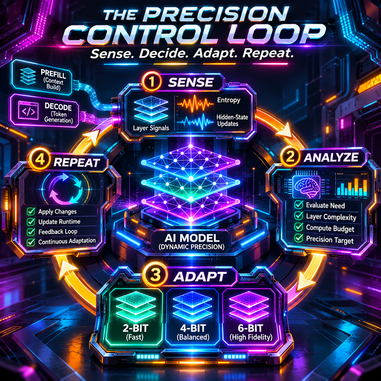
The loop senses two signals every step. The first is the normalized Shannon entropy of the next-token distribution over the top 10 logits. High entropy means the model is genuinely uncertain, and when it is uncertain a small quantization error can flip the token, so precision stays high. Low entropy means the continuation is predictable, so precision can drop.
The second signal is the magnitude of each layer's update to its hidden states. A layer that barely moves its representation does not need a fine-grained format. A layer with a large update is where the error lands.
Then it decides per layer, differently for the two phases. In prefill there is no entropy yet, so the loop runs on the hidden-state signal alone and looks for one large spike, flagged online when a layer's metric exceeds the mean by three standard deviations. Everything up to and including that spike layer runs at 6 bits, because that is where the prompt gets absorbed. After the spike the rule walks the stack one layer at a time, and each decision depends on the two layers before it. If both sat below the mean, the next layer drops one level. If both sat above, it rises one. The walk saturates at the top and bottom of the set, so it cannot run past 6 bits or below 2.
In decode the metric blends both signals, 0.7 for the hidden-state update and 0.3 for entropy, starts each layer at 4 bits, and moves four layers in the direction of the trend before it steps.
Then it steps and repeats, per layer, on every prefill and decode step. The precision set is 2, 4 and 6 bits, and the 2-bit tier applies to weights only. Two-bit activations and KV cache degrade accuracy badly enough that the authors exclude them, so the lowest rung is W2A4-KV4.
HOW THE BITS ACTUALLY MOVE
A runtime-switchable precision is worthless if switching costs more than it saves. That is the problem AutoFP solves, and the part most coverage will skip.
AutoFP keeps one base format, NVFP4, and derives the rest from it. The 6-bit level comes from mantissa refinement. Instead of storing a whole 6-bit tensor, each base value carries a 2-bit two's complement signed offset from negative two to positive one, stored separately, which moves it along the finer E2M3 grid on demand. The 2-bit level goes the other way, remapping the base's exponent bits into a quinary format.
Storing an offset for every element would eat the savings, so AutoFP refines only the subgroups where the error matters. It cuts each 16-element group into four 4-element subgroups and refines the ones above a normalized error threshold. Refining about half the weight subgroups recovers about 90 percent of the error reduction you would get by moving to 6 bits everywhere.
There are two implementations. One is kernels inside vLLM that execute all of it on stock NVFP4 Tensor Cores, which is why the GB300 result matters: 90 to 98 percent of NVFP4 decode throughput while running FP6-level accuracy, time to first token within 10 percent of the NVFP4 baseline and up to 1.4 times faster than a 6-bit baseline. The other is an accelerator whose vector MAC datapath executes all three formats natively, built as an extension of NVIDIA's MAGNet design with 256 processing elements, where one streamed activation meets two 2-bit weights, one NVFP4 weight, or one 6-bit weight per cycle.
Fewer bits per weight and per KV cache entry means more requests resident per chip, and resident requests are what you sell.
The paper is honest about the gap. AutoFP2 cannot serve as the stored base format, because reconstructing NVFP4 would cost more than the bandwidth it saves, so the 2-bit tier is an execution format, not a storage win. Do not read the 4.9 stored bits per weight as a 2-bit model.
WHY FLOP/S HID ALL OF THIS
Epoch AI published an Inference Performance Index on November 9 that scores accelerators on modeled agentic inference workloads instead of arithmetic. Its headline estimate is that the GB300 delivers about 25 times the H100's inference capacity per chip while offering only 2.5 times the 8-bit FLOP per second. Compare on FLOP/s alone and you understate the gap by a factor of ten.
The index models the two things that actually bind: how many requests a chip holds at once, and how fast each decodes, both governed by memory bandwidth and inter-chip communication rather than math throughput. It also shows the scale-up domain mattering: GB300 NVL72 models at about 1.9 times the capacity per GPU of B300 HGX on the same silicon, because 72 linked GPUs are a different machine from eight.
Same bill as the sizing argument we made in "Your GPU Scheduler Is Leaving 33 Points of Utilization on the Table." That piece covered what your scheduler wastes. This one covers what your format wastes.
My read, and this is opinion rather than anything the paper measured, is that precision switching lives on the correct side of that divide. It does not buy more arithmetic. It changes how much state you move per token and what each moved byte costs in energy. If you are sizing on FLOP/s you are already mis-sizing, and you will not have headroom to bank a 23 percent energy difference.
WHAT TO DO TODAY
- Audit your quantization against agentic multi-turn workloads, not a static benchmark. One fixed format for every layer means paying peak precision for work that does not need it, and a single-turn eval will not show you where, because demand moves across repeated prefills and long decodes.
- Separate KV cache precision from weight precision in your plan. They are different decisions with different error tolerances, and the KV cache is where your resident-request count moves.
- Build a per-layer precision map from your own traffic before you buy anything. Measure where entropy spikes and where hidden-state update magnitude sits across full agentic sessions, with tool calls, retries and growing context, not on one clean prompt.
- Run an accuracy audit at each candidate tier so the switch is defensible rather than vibes-based. A policy that drops a layer to 2 bits needs an eval that would catch it, and a calibration pass you ran once in August is not that eval.
- When you evaluate hardware, score it on modeled inference throughput rather than FLOP/s, and demand vendor numbers on agentic workloads at your output speed. The vendors publishing agentic figures are telling you which side of that divide they compete on.
THE UNCOMFORTABLE QUESTION
Your precision decision is a number in a config file you have not opened since the day you shipped. The hardware can now change that number every step, per layer, for up to 23 percent less energy at the same accuracy. What exactly are you waiting for?
Get More Articles Like This
Getting your AI agent setup right is just the start. I'm documenting every mistake, fix, and lesson learned as I build PhantomByte.
Subscribe to receive updates when we publish new content. No spam, just real lessons from the trenches.
Build Real AI Infrastructure
PhantomByte teaches you to build real AI infrastructure yourself: local AI stacks, autonomous agents, multi-agent orchestration, web scraping, and custom tools. Step-by-step PDF tutorials you download, follow, and deploy. No subscriptions. No fluff. Just skills that ship.